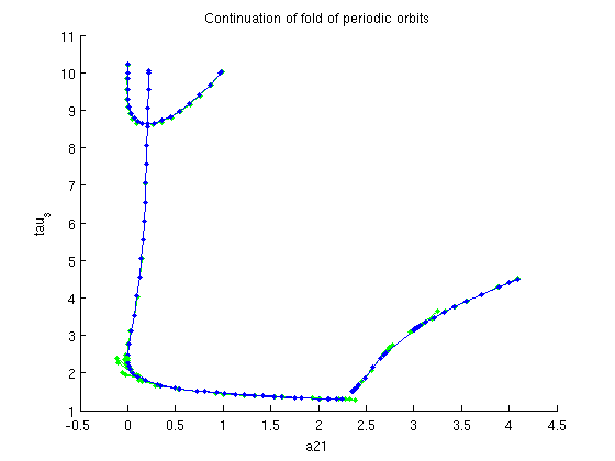
Continuation of folds of periodic orbits

The extension ddebiftool_extra_psol is able to continue local bifurcations of periodic orbits in two parameters. This demo shows how one can continue folds (saddle-nodes) of periodic orbits i nthe neuron problem. (requires running of demo1_psol.html first).

Add extension folder to path
Speed up computations by vectorization
Find initial guess
Initialize branch and set up extended system
Branch continuation
Extracting solution components
Stability of fold orbits
Save results (end of tutorial demo, but try also demo1_hcli.html)

Add extension folder to path

The extension is installed in a separate folder. In addition, a folder with utilities for user convenience is loaded.

addpath('../../ddebiftool_extra_psol/');
addpath('../../ddebiftool_utilities/');
%#ok<*ASGLU,*NOPTS,*NASGU>

Speed up computations by vectorization

The functions neuron_sys_rhs and neuron_sys_deri are not vectorized. In order to speed up computations we re-define neuron_sys_rhs, and replace neuron_sys_seri with the default finite-difference approximation

neuron_sys_rhs=@(xx,par)[...
    -par(1)*xx(1,1,:)+par(2)*tanh(xx(1,4,:))+par(3)*tanh(xx(2,3,:));....
    -par(1)*xx(2,1,:)+par(2)*tanh(xx(2,4,:))+par(4)*tanh(xx(1,2,:))];
vfuncs=set_funcs(...
    'sys_rhs',neuron_sys_rhs,...
    'sys_tau',@()[5,6,7],...
    'x_vectorized',true);

Find initial guess

For the branch computed in demo1_psol.html one fold occured at the maximal parameter value. So we extract its index indmax.

[dummy,indmax]=max(arrayfun(@(x)x.parameter(ind_a21),branch5.point));

Initialize branch and set up extended system

Then we call SetupPOfold to initialize the branch and to create the functions for the extended system. For the core DDE-Biftool routines the fold of periodic orbits is of the same type as a standard periodic orbit. However, the user-provided right-hand side has been extended (eg, foldfuncs.sys_rhs is different from funcs.sys_rhs). SetupPOfold has three mandatory parameters:

funcs containing the user-problem functions (in the demo: vfuncs),
branch, the branch on which the fold occurred (in the demo: branch5), and
ind, the index in branch.point near which the fold occurs (in the demo indmax).

Output (to be fed into br_contn):

foldfuncs: functions for the extended system (derived from funcs)
FPObranch: branch of folds of periodic orbits with two points

The other parameters are optional name-value pairs. Important are

'contpar': typically two integers ,the two continuation parameters,
'dir': in which direction the first step is taken), and
'step': the length of the first step. Note that name-value pairs are also passed on to fields of the branch structure: the output FPObranch inherits all fields from the input branch. Additional name-value argument pairs canbe used to change selected fields.

[foldfuncs,branch7]=SetupPOfold(vfuncs,branch5,indmax,'contpar',[ind_a21,ind_taus],...
    'dir',ind_taus,'print_residual_info',1,'step',0.01,'plot_measure',[],...
    'min_bound',[ind_a21,0],'max_bound',[ind_a21,4; ind_taus,10],...
    'max_step',[ind_a21,0.2; ind_taus,0.5]);

it=1, res=0.000574744
it=2, res=0.0083463
it=3, res=0.000139207
it=4, res=4.6582e-08
it=5, res=2.22616e-10
it=1, res=0.000267241
it=2, res=2.96116e-10
it=1, res=0.0699482
it=2, res=0.014741
it=3, res=6.29929e-06
it=4, res=2.28572e-10
it=1, res=0.000175272
it=2, res=8.75278e-10

Branch continuation

The output of SetupPOfold can be fed directly into br_contn to perform a branch continuation. Note that the computation is typically slower than a standard continuation of periodic orbits because the system dimension is twice as large and additional delays have been introduced.

figure(6);
branch7.method.point.print_residual_info=0;
branch7=br_contn(foldfuncs,branch7,100);
xlabel('a21');ylabel('tau_s');
title('Continuation of fold of periodic orbits');

BR_CONTN warning: boundary hit.

Extracting solution components

Since the fold continuation solves an extended system (with additional components) it does not make sense to compute the linear stability of the resulting orbits directly. However, foldfuncs has an additional field 'get_comp'. This is a function that extacts the components of the extended system that correspond to the solution of the original system. The output of get_comp is an array of periodic orbits that are located precisely on the fold.

pf_orbits=foldfuncs.get_comp(branch7.point,'solution');

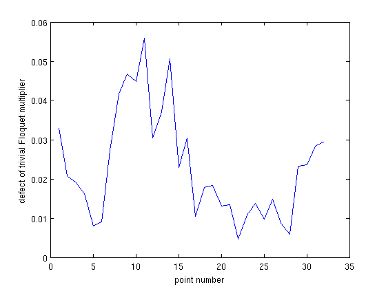
Stability of fold orbits

We compute Floquet multipliers for these orbits using the utility function GetStability(psol_array,...). Its optional inputs instruct it to ignore the two eigenvalues closest to 1 when computing stability. It also returns triv_defect which measures the distance of the supposedly trivial eigenvalues (as computed) to their correct values. GetStability needs the optional input 'funcs' if its first argument does not yet have a stability structure.

[nunst_pf,dom,triv_defect,pf_orbits]=GetStability(pf_orbits,'funcs',vfuncs,...
    'exclude_trivial',true,'locate_trivial',@(x)[1,1]);
fprintf('max number of unstable Floquet multipliers: %d\n',max(nunst_pf));
n_orbits=length(pf_orbits);
figure(16);
a21_pfold=arrayfun(@(x)x.parameter(4),branch7.point);
taus_pfold=arrayfun(@(x)x.parameter(7),branch7.point);
plot(1:n_orbits,triv_defect);
xlabel('point number');
ylabel('defect of trivial Floquet multiplier');

max number of unstable Floquet multipliers: 0

Save results (end of tutorial demo, but try also demo1_hcli.html)

save('demo1_POfold_results.mat')