DDE-Biftool demo -- Connecting orbits
% (c) DDE-BIFTOOL v. 3.1.1(20), 11/04/2014
This demo describes how to use DDE-Biftool to perform a bifurcation analysis on equations with several constant delays which exhibit connecting orbits.
As shown at the end of the neuron demo ../../neuron/html/demo1_hcli.html, one can compute connecting orbits using a direct method, when the delays are not state-dependent. In order to show the use of this method, we will now investigate a model of neural activity, described in [F Giannakopoulos and O. Oster, 1997].
Contents
- Initialization
- Differential equations
- Load pre-computed results of steady-state bifurcation analysis
- Figure: Bifurcations of equilibria in two-parameter plane
- Periodic orbits
- Figure: Period of the periodic orbits, as a function of the parameter q12.
- Figure: Time profile of last computed periodic orbit
- Conversion to homoclinic
- Figure: Time profile of uncorrected homoclinic
- Correction of initial homoclinic
- Figure: Remeshed and corrected profile of the same homoclinic orbit
- Creation of initial piece of branch
- Figure: Two-parameter bifurcation diagram in q12 and e1
- Second branch of homoclinic connections
- Figure: Two-parameter bifurcation diagram in q12 and e1
- Double homoclinic for symmetric system
- Figure: Evolution of parameter e1 vs. point number
- Figure: Phase portrait of the double homoclinic orbit for e1=-1.3.
- Takens-Bogdanov points
- Figure: Dominant eigenvalues of the saddle
- Refinement of homoclinic branch
- Figure: Dominant eigenvalues of the saddle
- End of demo - save results
Initialization
clear;                           % clear variables
format compact
close all;                       % close figures
addpath('../../ddebiftool/');    % add ddebiftool folder to path
%#ok<*ASGLU,*NOPTS,*NASGU>
Differential equations
The model is given as a two-dimensional system of differential equations
![$$
\begin{array}[t]{rcl}
\dot{x}_{1}(t)&=&-x_{1}(t)+q_{11}\frac{1}{1+\mathrm{e}^{-4x_{1}(t-\tau)}}
-q_{12}x_2(t-\tau) +e_1\\
\dot{x}_{2}(t)&=&-x_2(t)+q_{21}\frac{1}{1+e^{-4x_{1}(t-\tau)}}+e_2
\end{array}
$$](hom_demo_eq04885.png)
The parameters of the system are ![$[q_{11},q_{12}, q_{21}, e_1, e_2,\tau]$](hom_demo_eq53164.png) (in this order in the parameter vector). Our main bifurcation parameters are
(in this order in the parameter vector). Our main bifurcation parameters are  (q12) and
  (e1).
(e1).
g=@(xx)1/(1+exp(-4*xx(1,2)));
hom_rhs=@(xx,par)[...
    -xx(1,1)+par(1)*g(xx)-par(2)*xx(2,2)+par(4);...
    -xx(2,1)+par(3)*g(xx)+par(5)];
ind_tau=6;
ind_q12=2;
ind_e1=4;
funcs=set_funcs('sys_rhs',hom_rhs,'sys_tau',@()ind_tau);
Load pre-computed results of steady-state bifurcation analysis
The focus will be on the analysis of the homoclinic orbits in this system. Therefore, we will not repeat the standard bifurcation analysis. The reader is advised to run through the neuron demo ../../neuron/html/demo1.html to become more familiar with the analysis. For the purpose of this demo, we start at a point where branches of Hopf points and fold points have already been computed. The figure below shows branches of fold and Hopf points, plotted with respect to the two free parameters of the system,  and
and  . To obtain this figure, we first load the precomputed (and saved) branches from the file hom_demo.mat. We choose to plot the branches with respect to their default measure.
load('hom_demo_precomputed');
figure(1);
[xm,ym]=df_measr(0,fold_branch);
br_plot(fold_branch,xm,ym,':');
axis([1.28 1.62 -1.36 -1.24]);
hold on;
br_plot(hopf1_branch,xm,ym,'-.');
br_plot(hopf2_branch,xm,ym,'-.');
xlabel('q12');ylabel('e1');
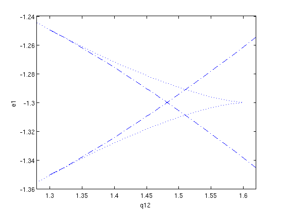
Figure: Bifurcations of equilibria in two-parameter plane
Branches of fold (dots) and Hopf (dashed) points.
Periodic orbits
We then select a Hopf point somewhere on the lower branch, and start the branch of periodic solutions that emanates from it. For this purpose, we create a branch of periodic solutions with two points. We choose to plot the period versus the free parameter while continuing, in order to visualize the approaching of the homoclinic orbit.
hopf=hopf1_branch.point(27);
[psol,stp]=p_topsol(funcs,hopf,1e-2,3,27)
psol =
         kind: 'psol'
    parameter: [2.6000 1.3428 1 -1.3398 -0.5000 1]
         mesh: [1x82 double]
       degree: 3
      profile: [2x82 double]
       period: 55.2714
stp =
         kind: 'psol'
    parameter: [0 0 0 0 0 0]
         mesh: [1x82 double]
       degree: 3
      profile: [2x82 double]
       period: 0
mpsol=df_mthod(funcs,'psol');
[psol,s]=p_correc(funcs,psol,ind_e1,stp,mpsol.point);
psol_branch=df_brnch(funcs,ind_e1,'psol');
psol_branch.point=psol;
[psol,stp]=p_topsol(funcs,hopf,2e-2,3,27);
[psol,s]=p_correc(funcs,psol,ind_e1,stp,mpsol.point);
psol_branch.point(2)=psol;
figure(2);clf;
[xm,ym]=df_measr(0,psol_branch);
ym.field='period';
ym.col=1;
ym.row=1;
psol_branch.method.continuation.plot_measure.x=xm;
psol_branch.method.continuation.plot_measure.y=ym;
[psol_branch,s,r,f]=br_contn(funcs,psol_branch,20);
xlabel('e1');ylabel('period');
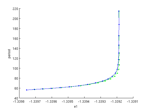
Figure: Period of the periodic orbits, as a function of the parameter q12.
figure(3);clf;
psol=psol_branch.point(end)
p_pplot(psol);
xlabel('time/period');ylabel('x1,x2');
psol =
         kind: 'psol'
    parameter: [2.6000 1.3428 1 -1.3392 -0.5000 1]
         mesh: [1x82 double]
       degree: 3
      profile: [2x82 double]
       period: 214.6858
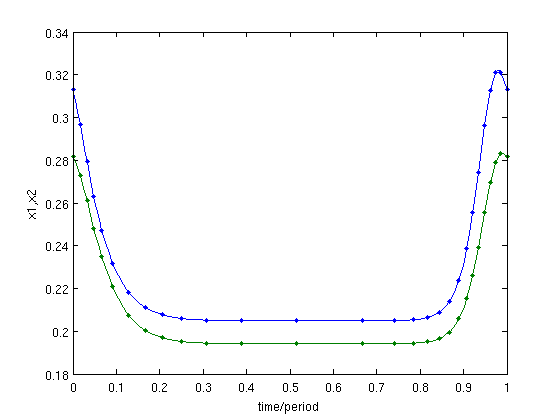
Figure: Time profile of last computed periodic orbit
The last point of this branch of periodic solutions has a large period, and is, thus, is close to a homoclinic orbit.
Conversion to homoclinic
We convert this point to a point of homoclinic type. This yields an (initially uncorrected) initial homoclinic profile. Note that the steady state is also uncorrected.
hcli=p_tohcli(funcs,psol)
figure(4);clf;
p_pplot(hcli);
xlabel('time/period');ylabel('x1,x2');
hcli =
         kind: 'hcli'
    parameter: [2.6000 1.3428 1 -1.3392 -0.5000 1]
         mesh: [1x79 double]
       degree: 3
      profile: [2x79 double]
       period: 182.1633
           x1: [2x1 double]
           x2: [2x1 double]
     lambda_v: 0.1691
     lambda_w: 0.1691
            v: [2x1 double]
            w: [2x1 double]
        alpha: -1
      epsilon: 5.2584e-06
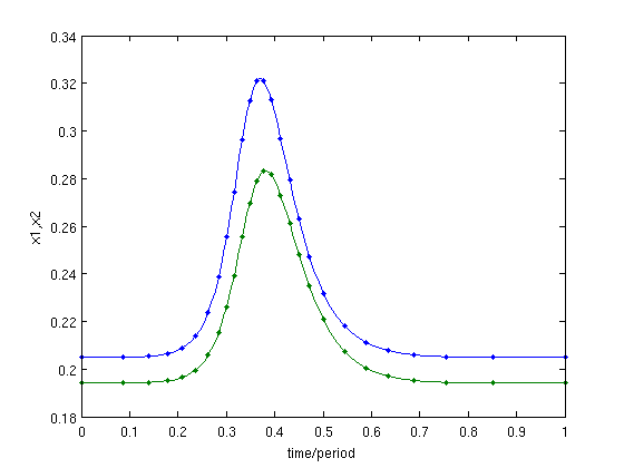
Figure: Time profile of uncorrected homoclinic
Correction of initial homoclinic
We correct this point (adjusting e1), after remeshing it on an adaptive mesh with 50 intervals. We plot this point before and after correction, see Figure below.
mhcli=df_mthod(funcs,'hcli');
[hcli,s]=p_correc(funcs,hcli,ind_e1,[],mhcli.point);  % correct
hcli=p_remesh(hcli,3,50);                             % remesh it and
[hcli,s]=p_correc(funcs,hcli,ind_e1,[],mhcli.point)   % correct it again
figure(5);clf;
p_pplot(hcli);                    % plot it after remeshing & correction
xlabel('time/period');ylabel('x1,x2');
hcli =
         kind: 'hcli'
    parameter: [2.6000 1.3428 1 -1.3392 -0.5000 1]
         mesh: [1x151 double]
       degree: 3
      profile: [2x151 double]
       period: 188.0558
           x1: [2x1 double]
           x2: [2x1 double]
     lambda_v: 0.1691
     lambda_w: 0.1691
            v: [2x1 double]
            w: [2x1 double]
        alpha: -1
      epsilon: 5.2584e-06
s =
     1
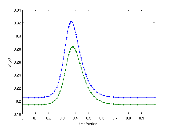
Figure: Remeshed and corrected profile of the same homoclinic orbit
Creation of initial piece of branch
We slightly change parameter value e1 of this homoclinic orbit, and compute a second homoclinic orbit for the new value of e1. With these two homoclinic solutions, we then create a branch, which is continued in two free parameters (e1 and q12). Finally we reverse the branch and continue it in the other direction.
hcli_br=df_brnch(funcs,[ind_q12, ind_e1],'hcli');
hcli_br.point=hcli;
hcli.parameter(ind_q12)=hcli.parameter(ind_q12)+6e-3;
[hcli,s]=p_correc(funcs,hcli,ind_e1,[],mhcli.point);
hcli_br.point(ind_q12)=hcli;
figure(1);
[hcli_br,s,r,f]=br_contn(funcs,hcli_br,85)
hcli_br=br_rvers(hcli_br);
[hcli_br,s,r,f]=br_contn(funcs,hcli_br,10)
xlabel('q12');ylabel('e1');
hcli_br =
       method: [1x1 struct]
    parameter: [1x1 struct]
        point: [1x71 struct]
s =
    70
r =
    16
f =
     0
hcli_br =
       method: [1x1 struct]
    parameter: [1x1 struct]
        point: [1x81 struct]
s =
    11
r =
     0
f =
     0
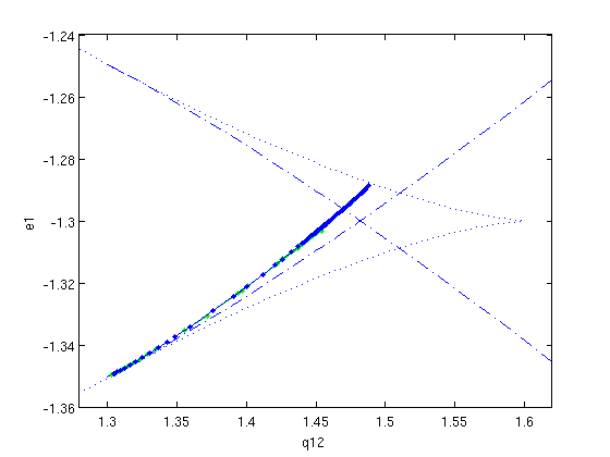
Figure: Two-parameter bifurcation diagram in q12 and e1
Now also showing one branch of homoclinic solutions (predictions and corrections).
Second branch of homoclinic connections
We do exactly the same for the second branch of Hopf points. Since the bifurcation diagram of this system is completely symmetric, we also approach homoclinic orbits when we jump onto the branches of periodic solutions emanating from those Hopf points. The commands are the same as in the above case, so we simply list them, without further explanation. We also do not plot the branch of periodic solutions while continuing.
% branch off from Hopf point 27 and continue periodic orbits to large
% period
hopf=hopf2_branch.point(27);
[psol,stp]=p_topsol(funcs,hopf,1e-2,3,27);
mpsol=df_mthod(funcs,'psol');
[psol,s]=p_correc(funcs,psol,ind_e1,stp,mpsol.point);
psol_branch=df_brnch(funcs,ind_e1,'psol');
psol_branch.point=psol;
[psol,stp]=p_topsol(funcs,hopf,2e-2,3,27);
[psol,s]=p_correc(funcs,psol,ind_e1,stp,mpsol.point);
psol_branch.point(2)=psol;
psol_branch.method.continuation.plot=0;
psol_branch.method.continuation.plot_progress=0;
[psol_branch,s,r,f]=br_contn(funcs,psol_branch,20);

% again the last point is close to a homoclinic
% so we convert it to a point of homoclinic type.

psol=psol_branch.point(end);
hcli=p_tohcli(funcs,psol);

% correct it
mhcli=df_mthod(funcs,'hcli');
[hcli,s]=p_correc(funcs,hcli,ind_e1,[],mhcli.point);

% remesh it and correct it
hcli=p_remesh(hcli,3,50);
[hcli,s]=p_correc(funcs,hcli,ind_e1,[],mhcli.point);

% we now continue this second  branch of homoclinic solutions in two-parameter
% space, and show this on the first figure.
hcli2_br=df_brnch(funcs,[ind_q12,ind_e1],'hcli');
hcli2_br.point=hcli;
hcli.parameter(ind_q12)=hcli.parameter(ind_q12)+6e-3;
[hcli,s]=p_correc(funcs,hcli,ind_e1,[],mhcli.point);
hcli2_br.point(2)=hcli;
figure(1);
hcli2_br=br_contn(funcs,hcli2_br,85);
hcli2_br=br_rvers(hcli2_br);
[hcli2_br,s,r,f]=br_contn(funcs,hcli2_br,10)
xlabel('q12');ylabel('e1');
hcli2_br =
       method: [1x1 struct]
    parameter: [1x1 struct]
        point: [1x80 struct]
s =
    11
r =
     0
f =
     0
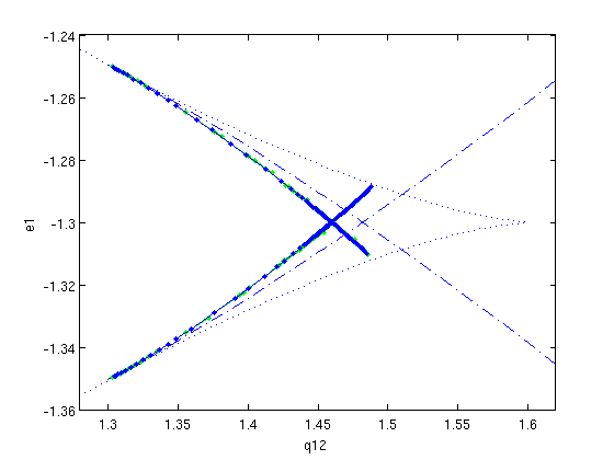
Figure: Two-parameter bifurcation diagram in q12 and e1
Now also showing two branches of homoclinic solutions (predictions and corrections). They both end at the branch of fold points, as the stability of the steady state changes at this point.
Double homoclinic for symmetric system
At e1=-1.3, a double homoclinic orbit exists. This is easily shown as follows. First, we look for the point on the branch where e1=-1.3. As the following figure shows, both branches intersect the horizontal line e1=-1.3. We find the intersection for both branches and name them i_hcli_intersect1 and i_hcli_intersect2.
[dum,i_hcli_intersect]=min(abs(arrayfun(@(p)p.parameter(ind_e1),hcli_br.point)+1.3));
[dum,i_hcli2_intersect]=min(abs(arrayfun(@(p)p.parameter(ind_e1),hcli2_br.point)+1.3));
i_max=max([i_hcli_intersect,i_hcli2_intersect])+20;
figure(6);
[xm,ym]=df_measr(0,hcli_br);
hold on;
br_plot(hcli2_br,[],ym);
br_plot(hcli_br,[],ym,'--');
plot([0 i_max],[-1.3 -1.3],'r-.',...
    i_hcli_intersect,-1.3,'kx',i_hcli2_intersect,-1.3,'kx');
axis([0,i_max,-1.31,-1.29]);
grid on
xlabel('point number');ylabel('e1');
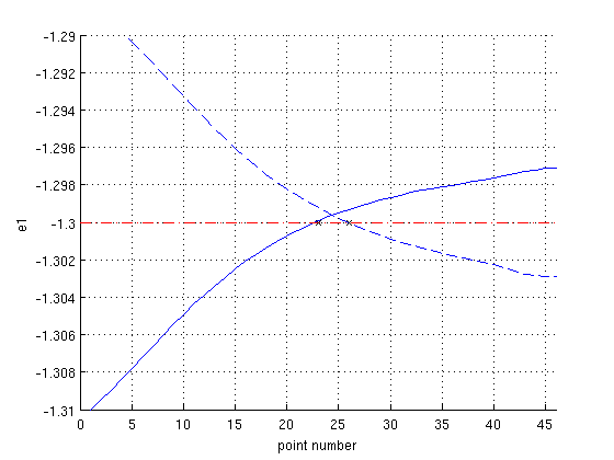
Figure: Evolution of parameter e1 vs. point number
along the first (dashed) and second (solid) branches of homoclinic orbits. Both approximate double homoclinic orbit are plotted below.
figure(7);
plot(hcli2_br.point(i_hcli2_intersect).profile(1,:),...
    hcli2_br.point(i_hcli2_intersect).profile(2,:));
hold on;
plot(hcli_br.point(i_hcli_intersect).profile(1,:),...
    hcli_br.point(i_hcli_intersect).profile(2,:));
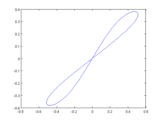
Figure: Phase portrait of the double homoclinic orbit for e1=-1.3.
The two loops are mirror images of each other.
Takens-Bogdanov points
Both branches of homoclinic orbits emanate from a Takens-Bogdanov bifurcation. As the amplitude of the homoclinic orbits along the branch goes to zero, the steady state approaches a Takens-Bogdanov-point. To illustrate this, the figure below shows the stability information of the last computed point on the branch. We see two small eigenvalues, but we are still at some distance from the Takens-Bogdanov point.
figure(8);
stst=p_tostst(funcs,hcli_br.point(end));
stst=stst(1);
mstst=df_mthod(funcs,'stst');
stst.stability=p_stabil(funcs,stst,mstst.stability);
p_splot(stst);
xlabel('\Re\lambda');ylabel('\Im\lambda');
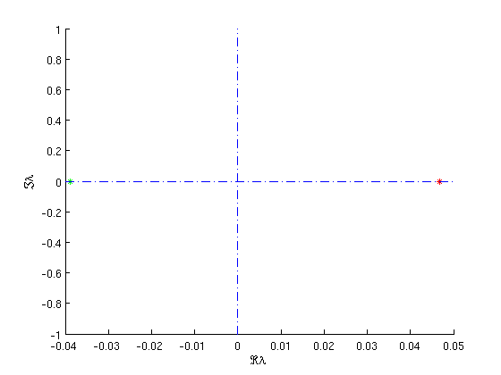
Figure: Dominant eigenvalues of the saddle
of the last point on the first branch of homoclinic orbits, near a Takens-Bogdanov bifurcation.
Refinement of homoclinic branch
In order to be able to continue the branch of homoclinic orbits closer to this Takens-Bogdanov point, we form a new branch, starting from the last point (with the profile remeshed on a finer mesh), and using a much smaller step size. If we would not do this, the steplength selection strategy (see manual) will take too large steps, resulting in a turnaround and a backward computation of the same branch.
We continue this new branch. During this continuation, it is possible that Matlab displays a warning concerning the near-singular character of the system being solved. This is an indication that we are close to the Takens-Bogdanov singularity. We then look again to the dominant eigenvalues of the last point, see figure below.
hcli=hcli_br.point(end);
hcli=p_remesh(hcli,3,70);
[hcli,s]=p_correc(funcs,hcli,ind_e1,[],mhcli.point);
to_tb_branch=df_brnch(funcs,[ind_q12,ind_e1],'hcli');
to_tb_branch.point=hcli;
hcli.parameter(ind_q12)=hcli.parameter(ind_q12)-1e-4;
hcli=p_remesh(hcli,3,70);
[hcli,s]=p_correc(funcs,hcli,ind_e1,[],mhcli.point);
to_tb_branch.point(2)=hcli;

to_tb_branch.method.continuation.plot=0;
to_tb_branch.method.continuation.plot_progress=0;
[to_tb_branch,s,r,f]=br_contn(funcs,to_tb_branch,40);

figure(9);
stst=p_tostst(funcs,to_tb_branch.point(end));
stst=stst(1);
mstst=df_mthod(funcs,'stst');
stst.stability=p_stabil(funcs,stst,mstst.stability);
p_splot(stst);
xlabel('\Re\lambda');ylabel('\Im\lambda');
Warning: Matrix is close to singular or badly scaled. Results may
be inaccurate. RCOND =  1.403289e-16.
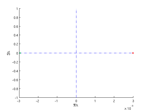
Figure: Dominant eigenvalues of the saddle
of the last point on the more accurate branch of homoclinic orbits, near a Takens-Bogdanov bifurcation.
End of demo - save results
save('hom_demo_results.mat');