Hopf bifurcation
(c) DDE-BIFTOOL v. 3.1.1(75), 31/12/2014
The eigenvalues of the linearized system along branches of equilibria indicate potential bifurcations. In this demo complex conjugate pairs of eigenvalues cross the imaginary axis, corresponding to Hopf bifurcations. The demo will proceed to continue two of these Hopf bifurcations in two system parameters  and
and  . This part requires to run demo1_stst.html first
Contents
- Locating the first Hopf point
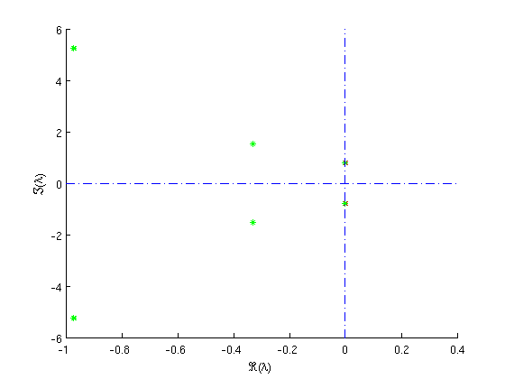
- Figure: eigenvalues at Hopf point
- Initialize and continue first Hopf bifurcation
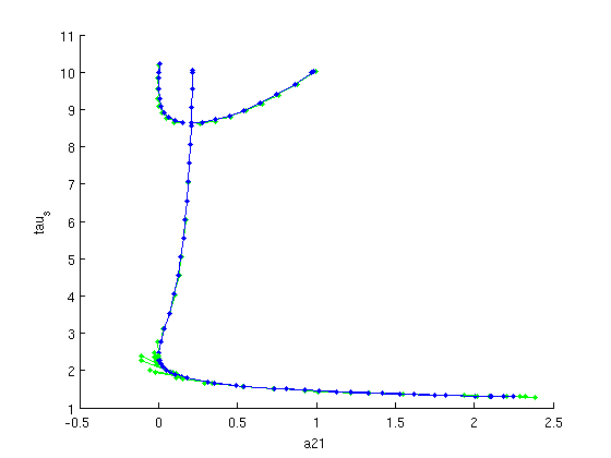
- Figure: Continuation (predictions and corrections) of Hopf bifurcation
- Hopf continuation and detecton of Takens-Bogdanov point
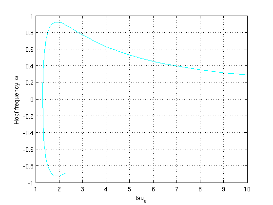
- Figures: Stability and frequency along first Hopf bifurcation
- Comments
- Switch to second Hopf bifurcation at double Hopf bifurcation
- Changing the Newton iteration and correction with other system parameter
- Continuation of second Hopf bifurcation
- Figure: Continuation (predictions and corrections) of both Hopf bifurcations
- Save and continue
%#ok<*ASGLU,*NOPTS,*NASGU>
%
Locating the first Hopf point
Where eigenvalue curves in the stability plot (see demo1_stst.html#stststability) cross the zero line, bifurcations occur. If we want to compute the Hopf bifurcation near  we need its point number. This is most easily obtained by plotting the stability versus the point numbers along the branch. We select the last point with positive eigenvalues and turn it into an (approximate) Hopf bifurcation point. We correct the Hopf point using appropriate method parameters and one free parameter (
 ). We then copy the corrected point to keep it for later use. Computing and plotting stability of the Hopf point clearly reveals the pair of purely imaginary eigenvalues.
ind_hopf=find(arrayfun(@(x)real(x.stability.l0(1))>0,branch1.point),1,'last');
hopf=p_tohopf(funcs,branch1.point(ind_hopf));
method=df_mthod(funcs,'hopf',flag_newhheur); % get hopf calculation method parameters:
method.stability.minimal_real_part=-1;
[hopf,success]=p_correc(funcs,hopf,ind_a21,[],method.point) % correct hopf
first_hopf=hopf;                    % store hopf point in other variable for later use
hopf.stability=p_stabil(funcs,hopf,method.stability); % compute stability of hopf point
figure(5); clf;
p_splot(hopf);                     % plot stability of hopf point
hopf =
         kind: 'hopf'
    parameter: [0.5 -1 1 0.807123224967979 0.2 0.2 1.5]
            x: [2x1 double]
            v: [2x1 double]
        omega: 0.78196516212093
success =
     1

Figure: eigenvalues at Hopf point
Characteristic roots at Hopf point: a pair of pure imaginary eigenvalues is clearly visible.
Initialize and continue first Hopf bifurcation
In order to follow a branch of Hopf bifurcations in the two parameter space  we again need two starting points. Hence we use the Hopf point already found and one perturbed in
  and corrected in
  , to start on a branch of Hopf bifurcations. For the free parameters,
  and
and  , we provide suitable intervals,
 ![$a_{21}\in[0,4]$](demo1_hopf_eq11829.png) and
and ![$\tau_s\in[0,10]$](demo1_hopf_eq54723.png) , and maximal stepsizes,
, and maximal stepsizes,  for
for  and
and  for
for  . We continue the branch on both sides by an intermediate order reversal and a second call to br_contn.
branch2=df_brnch(funcs,[ind_a21,ind_taus],'hopf'); % use hopf point as first point of hopf branch:
branch2.parameter.min_bound(1,:)=[ind_a21 0];
branch2.parameter.max_bound(1:2,:)=[[ind_a21 4]' [ind_taus 10]']';
branch2.parameter.max_step(1:2,:)=[[ind_a21 0.2]' [ind_taus 0.5]']';
branch2.point=hopf;

hopf.parameter(ind_taus)=hopf.parameter(ind_taus)+0.1; % perturb hopf point
[hopf,success]=p_correc(funcs,hopf,ind_a21,[],method.point); % correct hopf point, recompute stability
branch2.point(2)=hopf;                                 % use as second point of hopf branch:
figure(6); clf;
[branch2,s,f,r]=br_contn(funcs,branch2,40);            % continue with plotting hopf branch:
branch2=br_rvers(branch2);                             % reverse Hopf branch
[branch2,s,f,r]=br_contn(funcs,branch2,30);            % continue in other direction
xlabel('a21');ylabel('tau_s');
BR_CONTN warning: boundary hit.
BR_CONTN warning: boundary hit.
BR_CONTN warning: boundary hit.
BR_CONTN warning: boundary hit.

Figure: Continuation (predictions and corrections) of Hopf bifurcation
Predictions and corrections in the  -plane after computation of a first branch of Hopf bifurcations.
Hopf continuation and detecton of Takens-Bogdanov point
As we did not change continuation method parameters, predictions and corrections will be plotted during continuation. The final result is shown as figure. At the top, the branch hits the boundary  . To the right, however, it seemingly turned back onto itself. We compute and plot stability along the branch.
branch2=br_stabl(funcs,branch2,0,0);
figure(7); clf;
[xm,ym]=df_measr(1,branch2); % plot stability versus point number:
ym.subfield='l0';
br_plot(branch2,[],ym,'c');
ym.subfield='l1';
br_plot(branch2,[],ym,'b');
xlabel('point number along branch');ylabel('\Re(\lambda)');
% plot omega to identify 'false' turning point
% as Bogdanov-Takens point:
figure(8); clf;
[xm,ym]=df_measr(0,branch2);
ym
ym.field='omega';
ym.col=1;
xm
xm.col=7;
br_plot(branch2,xm,ym,'c');
grid on;
xlabel('tau_s');ylabel('Hopf frequency \omega');
ym =
       field: 'parameter'
    subfield: ''
         row: 1
         col: 7
        func: ''
xm =
       field: 'parameter'
    subfield: ''
         row: 1
         col: 4
        func: ''


Figures: Stability and frequency along first Hopf bifurcation
Real part of characteristic roots along the first branch of Hopf bifurcations (top). Bottom: The frequency of the Hopf bifurcation along the same branch.
Comments
If, during these computations we would have obtained warnings of the kind, TIME_H warning: h_min is reached, it would indicate that the time integration step required to obtain good approximations to the requested rightmost characteristic roots is too small. By default, characteristic roots are computed up to  . We also notice a double Hopf point on the left but nothing special at the right end, which could explain the observed turning of the branch. Plotting the frequency
  versus
  reveals what has happened, see figure. For small
  ,
,  goes through zero, indicating the presence of a Bogdanov-Takens point. The subsequent turning is a recomputation of the same branch with negative frequencies.
Switch to second Hopf bifurcation at double Hopf bifurcation
Selecting the double Hopf point we produce an approximation of the second Hopf point.
ind_hopf2=find(arrayfun(...
    @(x)numel(x.stability.l0)>=5&&real(x.stability.l0(5))<-1e-4,branch2.point),...
    1,'first');
hopf2=p_tohopf(funcs,branch2.point(ind_hopf2));
method.point.print_residual_info=1;
[hopf,success]=p_correc(funcs,hopf2,ind_a21,[],method.point) %fails
it=1, res=0.00834454
it=2, res=0.460349
it=3, res=0.0546203
it=4, res=0.00153245
it=5, res=1.96637e-05
hopf =
         kind: 'hopf'
    parameter: [0.5 -1 1 -0.0103306962446629 0.2 0.2 8.55313930216643]
            x: [2x1 double]
            v: [2x1 double]
        omega: 0.976827672655547
success =
     0
Changing the Newton iteration and correction with other system parameter
However, the correction fails. Printing residual information gives a list of the Newton iteration number and the norm of the residual. This reveals at least temporarily divergence of the correction process. Or we did not allow enough Newton iterations, or the free parameter is not so appropriate. We successfully try again using  as a free parameter.
[hopf,success]=p_correc(funcs,hopf2,ind_taus,[],method.point) % should now work
it=1, res=0.00834454
it=2, res=0.000618872
it=3, res=2.10605e-07
it=4, res=3.91466e-13
hopf =
         kind: 'hopf'
    parameter: [0.5 -1 1 0.206568018737126 0.2 0.2 8.63403521750747]
            x: [2x1 double]
            v: [2x1 double]
        omega: 0.915807193195807
success =
     1
Continuation of second Hopf bifurcation
Using the second Hopf point we compute the intersecting branch of Hopf points, depicted below. Setting plot_progress to zero disables intermediate plotting such that we see only the end result.
branch3=df_brnch(funcs,[ind_a21,ind_taus],'hopf');
branch3.parameter=branch2.parameter;
branch3.point=hopf;
% perturb and correct:
hopf.parameter(ind_a21)=hopf.parameter(ind_a21)-0.05;
method.point.print_residual_info=0;
format short;
[hopf,success]=p_correc(funcs,hopf,ind_taus,[],method.point);
branch3.point(2)=hopf; % use as second branch point:
% continue branch of hopf points on two sides:
branch3.method.continuation.plot_progress=0;
figure(6);
[branch3,s,f,r]=br_contn(funcs,branch3,100);
% reverse branch
branch3=br_rvers(branch3);
[branch3,s,f,r]=br_contn(funcs,branch3,100);
BR_CONTN warning: boundary hit.
BR_CONTN warning: boundary hit.

Figure: Continuation (predictions and corrections) of both Hopf bifurcations
Predictions and corrections in the  -plane after computation of second branch of Hopf bifurcations (superimposed on result of first Hopf bifurcation).
Save and continue
Continue with with periodic orbits demo1_psol.html or normal forms demo1_normalforms.html.
save('demo1_hopf_results.mat');