Continuation and stability of periodic orbits

DDE-biftool computes one-parameter families of periodic orbits (automatically determining their period) by solving periodic boundary-value problems approximately with collocation schemes. A typical starting point for a family of periodic orbits is a Hopf bifurcation. This demo requires demo1_hopf.html to have run beforehand.

Constructing an initial small-amplitude orbit near a Hopf bifurcation
Construction and continuation of branch
Figure: family of periodic orbits
Loss of accuracy along branch
Figures: Low accuracy solution profiles (top) and period (bottom) of periodic orbits
Stability of periodic orbits
Figures: Stability of periodic orbits at low accuracy
Refined computation with adaptive mesh
Homoclinic orbit
Save and continue

%#ok<*ASGLU,*NOPTS,*NASGU>
%

Constructing an initial small-amplitude orbit near a Hopf bifurcation

We use the first Hopf point we computed (first_hopf) to construct a small-amplitude (1e-2) periodic solution on an equidistant mesh of 18 intervals with piecewise polynomial degree 3. The steplength condition (returned by p_topsol) ensures the branch switch from the Hopf to the periodic solution as it avoids convergence of the amplitude to zero during corrections. Due to the presence of the steplength condition we also need to free one parameter, here $a_{21}$ .

intervals=18;
degree=3;
[psol,stepcond]=p_topsol(funcs,first_hopf,1e-2,degree,intervals);
% correct periodic solution guess:
method=df_mthod(funcs,'psol');
[psol,success]=p_correc(funcs,psol,4,stepcond,method.point)

psol = 
         kind: 'psol'
    parameter: [0.5000 -1 1 0.8072 0.2000 0.2000 1.5000]
         mesh: [1x55 double]
       degree: 3
      profile: [2x55 double]
       period: 8.0354
success =
     1

Construction and continuation of branch

The result, along with a degenerate periodic solution with amplitude zero is used to start on the emanating branch of periodic solutions, see figure below. We avoid adaptive mesh selection and save memory by clearing the mesh field. An equidistant mesh is then automatically used which is kept fixed during continuation. Simple clearing of the mesh field is only possible if it is already equidistant. This is the case here as p_topsol returns a solution on an equidistant mesh.

branch4=df_brnch(funcs,ind_a21,'psol'); % empty branch:
branch4.parameter.min_bound(1,:)=[ind_a21 0];
branch4.parameter.max_bound(1,:)=[ind_a21 5];
branch4.parameter.max_step(1,:)=[ind_a21 0.1];
% make degenerate periodic solution with amplitude zero at hopf point:
deg_psol=p_topsol(funcs,first_hopf,0,degree,intervals);
% use deg_psol and psol as first two points on branch:
deg_psol.mesh=[];
branch4.point=deg_psol;
psol.mesh=[];
branch4.point(2)=psol;
figure(9); clf;
[branch4,s,f,r]=br_contn(funcs,branch4,50); % compute periodic solutions branch
xlabel('a21');ylabel('amplitude');

Figure: family of periodic orbits

Branch of periodic solutions emanating from a Hopf point. The branch turns at the far right.

Loss of accuracy along branch

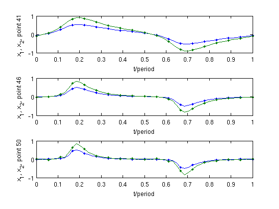
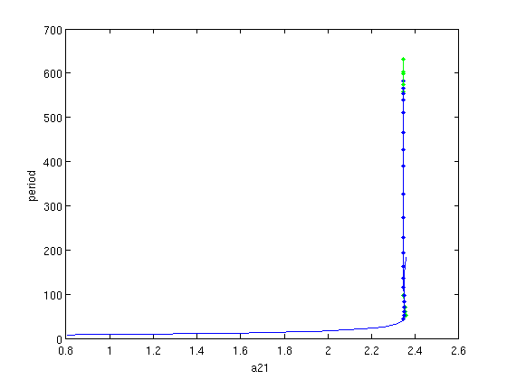
Notice how computing periodic solution branches takes considerably more computational time. Zooming shows erratic behaviour of the last computed branch points, shortly beyond a turning point, see figure below. Plotting some of the last solution profiles shows that smoothness and thus also accuracy are lost, see figure below. From a plot of the period along the branch we could suspect a homoclinic or heteroclinic bifurcation scenario.

ll=length(branch4.point);
figure(10); clf;
subplot(3,1,1);
p_pplot(branch4.point(ll-10));
xlabel('t/period');ylabel(sprintf('x_1, x_2, point %d',ll-10));
subplot(3,1,2);
p_pplot(branch4.point(ll-5));
xlabel('t/period');ylabel(sprintf('x_1, x_2, point %d',ll-5));
subplot(3,1,3);
p_pplot(branch4.point(ll-1));
xlabel('t/period');ylabel(sprintf('x_1, x_2, point %d',ll-1));
figure(11); clf;
[xm,ym]=df_measr(0,branch4);
ym
ym.field='period';
ym.col=1;
br_plot(branch4,xm,ym,'b');% look at the period along the branch:
axis([2.2 2.36 20 170]);
xlabel('a21');ylabel('period');

ym = 
       field: 'profile'
    subfield: ''
         row: 1
         col: 'ampl'
        func: ''

Figures: Low accuracy solution profiles (top) and period (bottom) of periodic orbits

Three solution profiles using equidistant meshes (top), and period (bottom) along the branch of periodic solutions.

Stability of periodic orbits

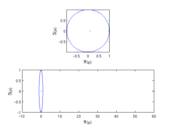
We compute and plot the stability (Floquet multipliers) just before and after the turning point. The second spectrum is clearly unstable but no accurate trivial Floquet multiplier is present at 1.

psol=branch4.point(ll-11);
psol.stability=p_stabil(funcs,psol,method.stability);
figure(12); clf;
subplot(2,1,1);
p_splot(psol);
axis image;
psol=branch4.point(ll-8);
psol.stability=p_stabil(funcs,psol,method.stability);
subplot(2,1,2);
p_splot(psol);

Figures: Stability of periodic orbits at low accuracy

Floquet multipliers for a periodic solutions before (top) and just after (bottom) the turning point visible in figure.

Refined computation with adaptive mesh

We recompute the branch using adaptive mesh selection (with reinterpolation and additional corrections) after correcting every point, see figure. Increasing mesh sizes and using adaptive mesh selection also improves the accuracy of the computed Floquet multipliers.

psol=branch4.point(ll-12:ll-11); %refine these two points
intervals=40;
degree=4;
psol=arrayfun(@(p)p_remesh(p,degree,intervals),psol); % refine
method.point.adapt_mesh_after_correct=1;
method.point.newton_max_iterations=7;
method.point.newton_nmon_iterations=2;
psol=arrayfun(@(p)p_correc(funcs,p,[],[],method.point),psol) %correct
branch5=branch4;
branch5.point=psol;
branch5.method=method;
[xm,ym]=df_measr(0,branch5);
ym.field='period';
ym.col=1;
figure(11); axis auto; hold on;
branch5.method.continuation.plot_measure.x=xm;
branch5.method.continuation.plot_measure.y=ym;
[branch5,s,f,r]=br_contn(funcs,branch5,25);
xlabel('a21');ylabel('period');

psol = 
1x2 struct array with fields:
    kind
    parameter
    mesh
    degree
    profile
    period

Homoclinic orbit

Plotting of a point clearly shows the (double) homoclinic nature of the solutions.

%<html><a name=longperiod></a></html>
%
figure(13); clf;
subplot(2,1,1);
indmax0=length(branch5.point);
psol=branch5.point(indmax0-6);
plot(psol.mesh,psol.profile);
xlabel('t/period');ylabel('x1, x2');
subplot(2,1,2);
psol1=p_remesh(psol,degree,0:0.001:1);
psol2=p_remesh(psol,degree,(0:0.001:1)+0.02);
plot(psol1.profile',psol2.profile');
xlabel('x1');ylabel('x2');
psol.period

ans =
  389.6531

Save and continue

with homoclinic connections demo1_hcli.html or folds of periodic orbits demo1_POfold.html

save('demo1_psol_results.mat');